根据网易的xgboost课程,结合他们的pdf文件以及python代码写的一篇博客
1 | from xgboost import XGBRegressor as XGBR |
导入参数
1 | import warnings |
对模型进行训练
1 | reg = XGBR(n_estimators=100).fit(Xtrain,Ytrain) # 参数实例化 |
0.9050988968414799
1 | MSE(Ytest,reg.predict(Xtest)) # 均方误差 |
8.830916343629323
1 | reg.feature_importances_ #模型重要性负数,每一个特征值的权重 |
array([0.01902167, 0.0042109 , 0.01478316, 0.00553537, 0.02222196,
       0.37914088, 0.01679686, 0.0469872 , 0.04073574, 0.05491759,
       0.06684221, 0.00869464, 0.3201119 ], dtype=float32)
交叉验证,使用没有训练的模型
1 | reg = XGBR(n_estimators=100) |
0.7995062821902295
1 | CVS(reg,Xtrain,Ytrain,cv=5,scoring='neg_mean_squared_error').mean() #负均方误差 |
-16.215644229762717
模型对比
1 | rfr = RFR(n_estimators=100) # 使用随机森林进行对比 |
0.8010385665818835
1 | lr = LinearR() # 线性回归 |
0.6835070597278076
1 | reg = XGBR(n_estimators=10,verbosity=0) |
-18.633733952333067
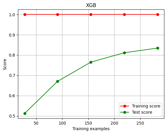
绘制学习曲线
1 | def plot_learning_curve(estimator,title, X, y, |
1 | cv = KFold(n_splits=5,shuffle=True,random_state=42)# 交叉验证模式 |
1 | plot_learning_curve(XGBR(n_estimators=100,random_state=420),"XGB",Xtrain,Ytrain,ax=None,cv=cv) |
进行调参
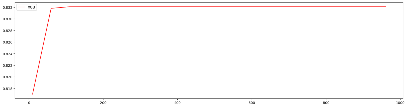
绘制学习曲线观察n_estimators的影响
对10~1010进行计算
1 | axisx = range(10,1010,50) |
160 0.8320776498992342
方差与泛化误差
泛化误差:E(f;D),方差:var,偏差:bias,噪声:ξ。
$~~~~~~~~~~~~~~~~~~~~~~~~~~~~~~~~~~~~~$E(f;D) = bias² + var + ξ²
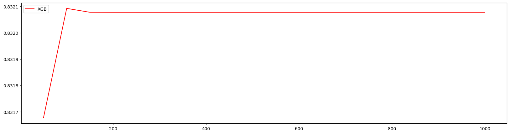
1 | axisx = range(50,1050,50) |
100 0.8320924293483107 0.005344212126112929
100 0.8320924293483107 0.005344212126112929
100 0.8320924293483107 0.005344212126112929 0.03353716440826495
细化学习曲线,找到最佳n_estimators
1 | axisx = range(50,200,10) # 将范围缩小 |
100 0.8320924293483107 0.005344212126112929
100 0.8320924293483107 0.005344212126112929
100 0.8320924293483107 0.005344212126112929 0.03353716440826495
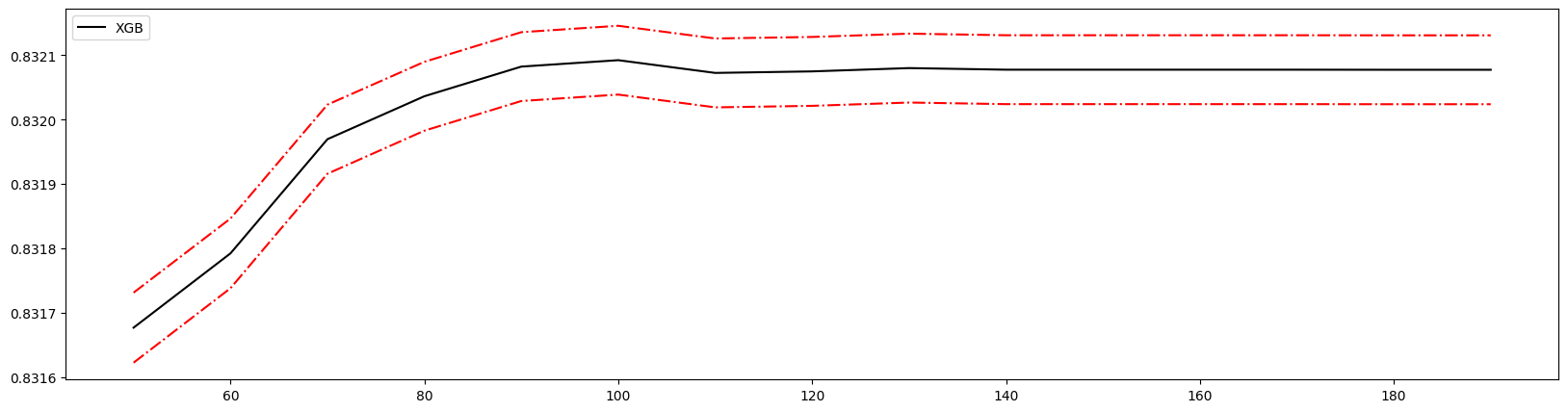
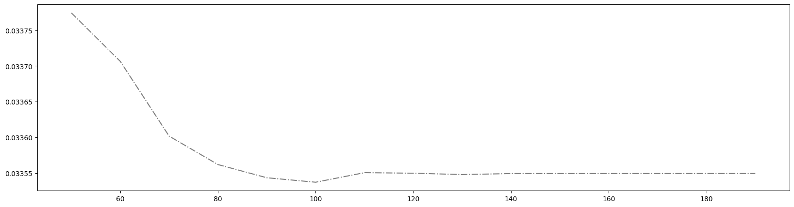
得到最佳取值为100。
有放回随机抽样,重要参数subsample
了解有放回随机抽样
$~~~~~~~$第一次随机从原始数据集中进行随机抽取,将其进行建模。把模型结果,即预测错误的样本反馈回原始数据集,增加其权重。然后循环此过程,不断修正之前判断错误的样本。一定程度上提升模型准度。
$~~~~~~~$在sklearn和xgboost中,使用subsample作为随机抽样参数,范围为(0,1],默认为一,为抽取占原数据比例。
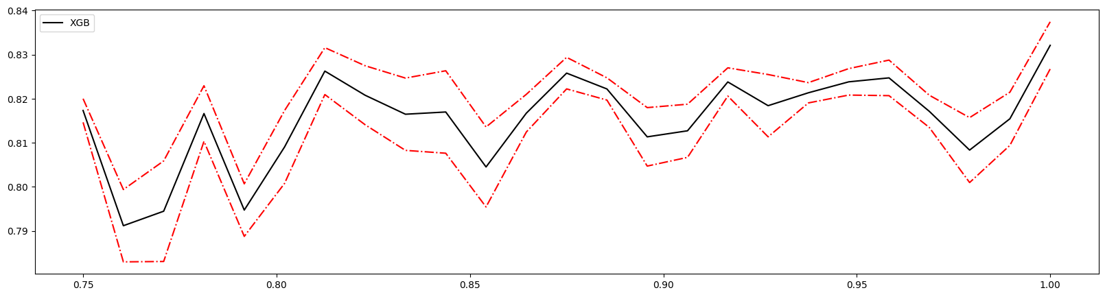
进行学习曲线分析
1 | axisx = np.linspace(0.75,1,25)# 随机选取数值,多次调整,缩减范围 |
1.0 0.8320924293483107 0.005344212126112929
0.9375 0.8213387927010547 0.0023009355462403113
1.0 0.8320924293483107 0.005344212126112929 0.03353716440826495
1 | reg = XGBR(n_estimators=100,subsample=0.9375,random_state=420).fit(Xtrain,Ytrain) |
0.9175041345374846
1 | MSE(Ytest,reg.predict(Xtest)) |
7.676560781152187
显然优于没有设置时的模型。如果模型准确率降低则取消使用此参数。
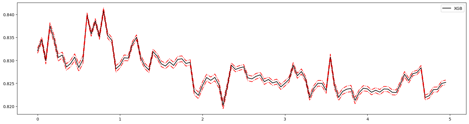
将n_estimators和subsample一起进行训练取得最优解
1 | axisx_sub = np.linspace(0.75,1,25) |
160 0.9583333333333333 0.8432917907566264 0.004614845818885538
50 0.9479166666666666 0.8339831443137825 0.003529311838690004
190 0.9479166666666666 0.842287142171737 0.004044787817216516 0.028918133341574434
迭代决策树,重要参数eta
参数eta为迭代决策树的步长。
迭代树公式为:
$~~~~~~~~~~~~~~~~~~~~~~~~~$$y_i^{k+1} = y_i^k + ŋf_{k+1}^{x_i}$
eta即为ŋ,也称为学习率,取值范围为[0,1]。在xgboost中默认为0.3,在sklearn中为0.1。
1 | # 评分函数 |
1 | axisx = np.arange(0.05,1,0.05) |
0.35000000000000003 0.8398273910404873
1 | reg = XGBR(n_estimators=190,subsample=0.9479166666666666,random_state=420,eta=0.35).fit(Xtrain,Ytrain) |
0.8954798646898599
1 | MSE(Ytest,reg.predict(Xtest)) |
9.726004655677164
发现并没有提升,反而下降。eta一般作为模型训练时间的调整指标,如果模型没有错误,一般都会收敛,eta影响并不算大。根据训练经验,eta取值一般在0.1左右
XGBoost
选择弱评估器:booster参数
$~~~~~~~$在sklearn中为booster参数,在xgboost中为xgb_model。用于选择弱评估器,可以输入的值有:gbtree、gblinear和dart。gbtree为梯度提升树,gblinear为线性模型,dart为抛弃提升树,比梯度提升树有更好的放过拟合功能。在xgboost中必须用param传入参数。
1 | for booster in ["gbtree","gblinear","dart"]: |
gbtree
0.9199261332157886
gblinear
0.6525347637145433
dart
0.9261191829728914
目标函数:objective
$~~~~~~~$在xgboost中使用目标函数来替代传统损失函数。xgb的目标函数可以写为:损失函数+模型复杂度。
$~~~~~~~~~~~~~~~~~~~$ $Obj = \sum_{i=1}^m l(y_i , y_i’) + \sum_{k=1}^K \Omega(f_k)$
$~~~~~~~$第一项为损失函数,用来评估模型准确度。第二项为模型复杂度和树结构复杂度有直接联系,运用此函数添加在损失函数之后,可以使模型在准确的同时用最少的运算时间。当两者都最小,则平衡了模型效果和工程能力,使XGBoost运算又快又准。
$~~~~~~~$方差用于评估模型稳定性,偏差用于评估模型的准确率。对应此目标函数。第一项衡量的是偏差,第二项则衡量方差。所以此目标函数也表示方差偏差平衡,也就是泛化误差。
$~~~~~~~$对于xgboost,可以选择第一项的使用函数。在xgboost中参数为obj(也可以写成object),在sklearn中为objective。在xgb.train() 和xgb.XGBClassifier() 中默认为 binary:logistic,在xgb.XGBRegressor() 中默认为 reg:linear 。
常用的参数有:
| 输入 | 使用的损失函数 |
|---|---|
| reg:linear | 使用线性回归的损失函数,均方误差,回归时使用 |
| binary:logistic | 使用逻辑回归的损失函数,对数损失log_loss,二分类时使用 |
| binary:hinge | 使用支持向量机的损失函数,Hinge Loss,二分类时使用 |
| multi:softmax | 使用softmax损失函数,多分类时使用 |
现在推荐使用reg:squarederror来代替reg:linear。
$~~~~~~~$使用xgboost库来进行训练的流程:
$xgb.DMatrix() -> param={} -> bst=xgb.train(param) -> bst.predict()$
$ 读取数据->设置参数->训练模型->预测结果 $
使用sklearn进行xgboost
1 | reg = XGBR(n_estimators=190,random_state=420,eta=0.1 |
0.9261191829728914
1 | MSE(Ytest,reg.predict(Xtest)) |
6.874897054416443
使用xgboost库
1 | import xgboost as xgb |
使用类DMatrix读取数据
1 | dtrain = xgb.DMatrix(Xtrain,Ytrain) # 特征矩阵和标签都进行一个传入 |
如果想要查看数据,可以在导入数据进入DMatrix之前在pandas中查看
1 | import pandas as pd |
| 0 | 1 | 2 | 3 | 4 | 5 | 6 | 7 | 8 | 9 | 10 | 11 | 12 | |
|---|---|---|---|---|---|---|---|---|---|---|---|---|---|
| 0 | 0.03041 | 0.0 | 5.19 | 0.0 | 0.515 | 5.895 | 59.6 | 5.6150 | 5.0 | 224.0 | 20.2 | 394.81 | 10.56 |
| 1 | 0.04113 | 25.0 | 4.86 | 0.0 | 0.426 | 6.727 | 33.5 | 5.4007 | 4.0 | 281.0 | 19.0 | 396.90 | 5.29 |
| 2 | 10.23300 | 0.0 | 18.10 | 0.0 | 0.614 | 6.185 | 96.7 | 2.1705 | 24.0 | 666.0 | 20.2 | 379.70 | 18.03 |
| 3 | 0.17142 | 0.0 | 6.91 | 0.0 | 0.448 | 5.682 | 33.8 | 5.1004 | 3.0 | 233.0 | 17.9 | 396.90 | 10.21 |
| 4 | 0.05059 | 0.0 | 4.49 | 0.0 | 0.449 | 6.389 | 48.0 | 4.7794 | 3.0 | 247.0 | 18.5 | 396.90 | 9.62 |
| ... | ... | ... | ... | ... | ... | ... | ... | ... | ... | ... | ... | ... | ... |
| 349 | 0.03871 | 52.5 | 5.32 | 0.0 | 0.405 | 6.209 | 31.3 | 7.3172 | 6.0 | 293.0 | 16.6 | 396.90 | 7.14 |
| 350 | 0.12650 | 25.0 | 5.13 | 0.0 | 0.453 | 6.762 | 43.4 | 7.9809 | 8.0 | 284.0 | 19.7 | 395.58 | 9.50 |
| 351 | 6.96215 | 0.0 | 18.10 | 0.0 | 0.700 | 5.713 | 97.0 | 1.9265 | 24.0 | 666.0 | 20.2 | 394.43 | 17.11 |
| 352 | 0.09164 | 0.0 | 10.81 | 0.0 | 0.413 | 6.065 | 7.8 | 5.2873 | 4.0 | 305.0 | 19.2 | 390.91 | 5.52 |
| 353 | 5.58107 | 0.0 | 18.10 | 0.0 | 0.713 | 6.436 | 87.9 | 2.3158 | 24.0 | 666.0 | 20.2 | 100.19 | 16.22 |
354 rows × 13 columns
写明参数
1 | param = {'objective':'reg:squarederror' |
类train,可以直接导入的参数是训练数据,树的数量,其他参数都需要通过params来导入
1 | bst = xgb.train(param, dtrain, num_round) |
使用接口
1 | preds = bst.predict(dtest) |
导入sklearn库进行R方和均方误差评估
1 | from sklearn.metrics import r2_score |
0.9264166709056179
1 | MSE(Ytest,preds) |
6.8472146465232635
通过对比发现xgboost库本身是优于sklearn库里xgboost的
求解目标函数
$~~~~~~~~~~~~~~~~~~~~~~~~~~~~~~~~~~~~~~~~~~~~$ $Obj = \sum_{i=1}^m l(y_i , y_i’) + \sum_{k=1}^K \Omega(f_k) $
简化目标函数,将损失函数转换,使用泰勒展开
$~~~~~~~~~~~~~~~~~~~~~~~~~~~~~~~~~~~~~~$ $\sum_{i=1}^m[f_t(x_i)g_i + \frac{1}{2} (f_t(x_i))^2 h_i] + \Omega(f_t)$
$g_i$和$h_i$为在损失函数上对$y_i^{t-1}$的一阶导数和二阶导数
参数化决策树$f_k(x)$:参数alpha,lambda
$f_k(x_i)$是每个叶子节点的回归值
所以回归结果为$y_i^k = \sum_{k}^K f_k(x_i)$
使用$q(x_i)$表示样本$x_i$的叶子节点,并用$w_{q(x_i)}$表示第k棵树上第$q(x_i)$叶子节点的分数。所以有:
$~~~~~~~~~~~~~~~~~~~~~~~~~~~~~~~~~~~~~~~~~~~~~~~~~~~~~~~~~~~~~~~~~~~~~$ $f_k(x_i) = w_{q(x_i)}$
于是得到复杂度计算公式:
$$\Omega(f) = \gamma T + 正则项$$
利用正则项来控制xgboost的过拟合情况。xgb中参数为alpha和lambda取值为[0,∞],再sklearn中参数为reg_alpha和reg_lambda取值范围和xgboost一样。默认优先使用lambda参数,如果需要alpha参数,可以使用之前的方法将两个参数放在一起来找到最好取值。
1 | #使用网格搜索来查找最佳的参数组合 |
56:42:172725


7.395192625759336
寻找最佳树结构:求解$\omega$与T
通过之前的推到得到新的目标函数:
$~~~~~~~~~~~~~~~~~~~~~~~~~~~~~~~~~~~~~~~~~~~~~~~~$ $ \sum_{i=1}^m[f_t(x_i)g_i+\frac{1} {2} (f_t(x_i)^2 h_i)] + \Omega(f_t) $
$$ = \sum_{i=1}^m[w_{q(x_i)}g_i+\frac{1}{2} w_{q(x_i)}^2 h_i] + \gamma T + \frac{1}{2}\lambda\sum_{j=1}^T w_j^2$$
有:
$$\sum_{i=1}^m w_q(x_i) * g_i = \sum_{j=1}^T(w_j\sum_{i∊I_j} g_i)$$
整理合并后得到:
$$= \sum_{j=1}^T [w_j\sum_{i∊I_j}g_i + \frac{1}{2}w_j^2 (\sum_{i∊I_j} h_i + \lambda)] + \gamma T $$
我们定义 $G_j = \sum_{i∊I_j}g_i , H_j = \sum_{i∊I_j}h_i $
最终得到:
$$Obj^t = \sum_{j=1}^T [w_jG_j + \frac{1}{2} w_j^2(H_j + \lambda)] + \gamma T$$
$$F^*(w_j) = w_jG_j + \frac{1}{2}w_j^2(H_j + \lambda)$$
然后对$F^*$进行偏导求取极小值得到:
$$w_j = -\frac{G_j}{H_j + \lambda}$$
得到:
$$Obj^t = -\frac{1}{2}\sum_{j=1}^T \frac{G_j^2}{H_j + \lambda} + \gamma T$$
寻找最佳分支
使用贪婪算法求得,与求解最佳决策树相似,只需要将信息熵修改为目标函数来衡量树的优劣。
将创建前的树的结构分数与创建节点后的结构分数做差得出的式子称为Gain,需要取得最大Gain来创建新节点,与决策树取得最大信息增益创建节点同理。
$$Gain = \frac{1}{2}[\frac{G_L^2}{H_L + \lambda} + \frac{G_R^2}{H_R + \lambda} - \frac{(G_L + G_R)^2}{H_L + H_R + \lambda}] - \gamma$$
让树停止生长:参数 $\gamma$
gamma越大算法越保守,叶子数量越少,算法复杂度越低。在xgboost和sklearn参数名都为gamma都默认为0,取值为[0,+∞)。
1 | # 测试与之前方法一致 |
0.8 0.840869937975637 0.005891402581053541
4.55 0.8270850835330702 0.004605425533747813
0.6000000000000001 0.8398453482504387 0.004660990862047279 0.030310503339070552
可以看到无法观测出趋势,所以引入新的工具:xgboost.cv。
1 | import xgboost as xgb |
1 | #设定参数 |
1 | #使用类xgb.cv |
00:00:565108
1 | #查看结果 |
| train-rmse-mean | train-rmse-std | test-rmse-mean | test-rmse-std | |
|---|---|---|---|---|
| 0 | 17.105578 | 0.129116 | 17.163215 | 0.584297 |
| 1 | 12.337973 | 0.097557 | 12.519736 | 0.473458 |
| 2 | 8.994071 | 0.065756 | 9.404534 | 0.472310 |
| 3 | 6.629481 | 0.050323 | 7.250335 | 0.500342 |
| 4 | 4.954406 | 0.033209 | 5.920812 | 0.591874 |
| ... | ... | ... | ... | ... |
| 185 | 0.001209 | 0.000110 | 3.669902 | 0.857671 |
| 186 | 0.001209 | 0.000110 | 3.669902 | 0.857671 |
| 187 | 0.001209 | 0.000110 | 3.669902 | 0.857671 |
| 188 | 0.001209 | 0.000110 | 3.669902 | 0.857671 |
| 189 | 0.001209 | 0.000110 | 3.669902 | 0.857671 |
190 rows × 4 columns
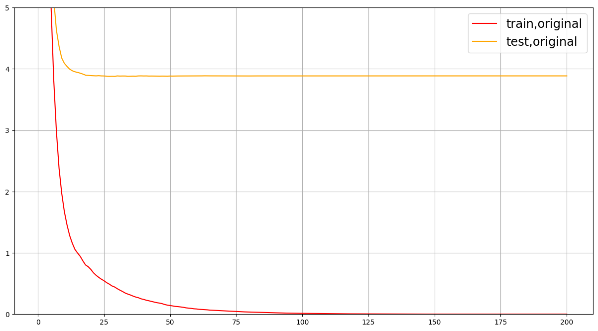
1 | plt.figure(figsize=(20,5)) |
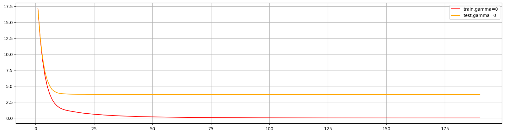
xgboost自带了很多评估指标:
| 指标 | 含义 |
|---|---|
| rmse | 回归用,调整后的均方误差 |
| mae | 回归用,绝对平均误差 |
| logloss | 二分类用,对数损失 |
| mlogloss | 多分类用,对数损失 |
| error | 分类用,分类误差,等于1-准确率 |
| auc | 发类用,auc面积 |
1 | param1 = {'silent':True |
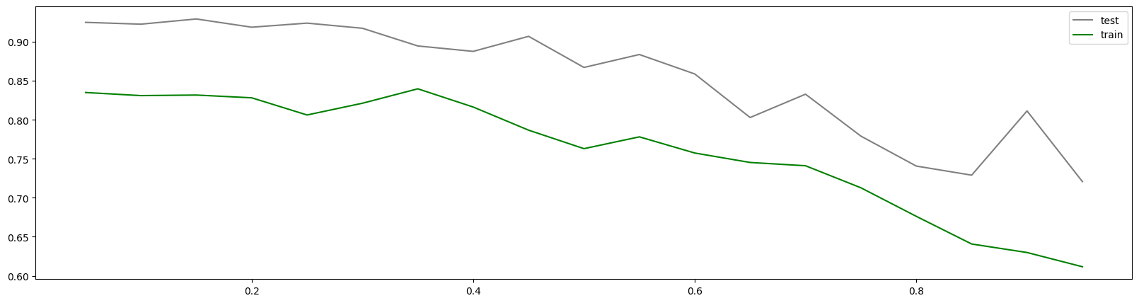
这个图形可以判断出num_round的大致数目,在75以后,模型趋于平稳,所以可以适量减少树的数量。
还可以通过此图两条线的差值看出模型出现了过拟合,可以进行修正。
1 | # 设置不同的gamma |
00:00:551680
1 | time0 = time() |
00:00:637867
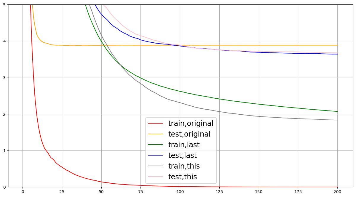
1 | plt.figure(figsize=(20,5)) |
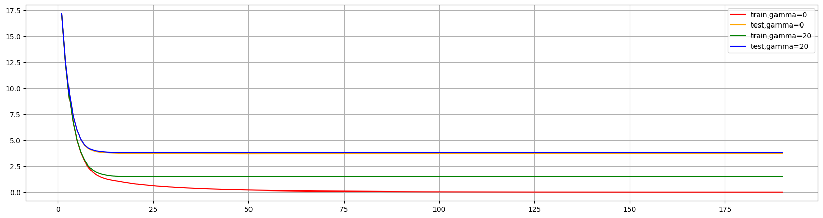
可以看出调高gamma后,大幅缩小了差异,减少了过拟合情况。但是是通过降低对训练集的表现来降低过拟合。来限制学习从而提升泛化能力。
使用乳腺癌数据集来看看xgboost分类模型中gamma的表现
1 | from sklearn.datasets import load_breast_cancer |
1 | time0 = time() |
00:00:158470
1 | time0 = time() |
00:00:207306
1 | plt.figure(figsize=(20,5)) |
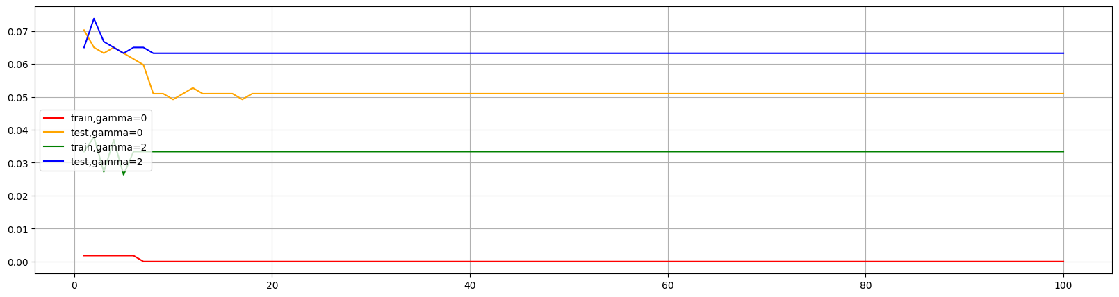
发现提高gamma后不仅减少了训练集表现,也降低了测试集的表现。所以可以适当减小gamma值,使得测试集表现不变而降低训练集,使过拟合情况缓解。
通过时间测试可以看出xgboost.cv的速度远远高于学习曲线,所以尽量使用cv来进行参数调节。
过拟合参数:剪枝参数与回归模型调参
| 参数含义 | xgboost:默认值 | sklearn:默认值 |
|---|---|---|
| 树的最大深度 | max_depth:6 | max_depth:6 |
| 每次生成树时随机抽样特征比例 | colsample_bytree:1 | colsample_bytree:1 |
| 每次生成树的一层时随机抽样比例 | colsample_bylevel:1 | colsample_bylevel:1 |
| 每次生成一个叶子节点时随机抽样特征比例 | colsample_bynode:1 | NONE |
| 一个叶子节点上所需要的最小$h_i$类似样本权重 | min_child_weight:1 | min_child_weight:1 |
一般调整模型先选择n_estimators和eta,如何使用gamma和max_depth来调整过拟合情况。
1 | dfull = xgb.DMatrix(x,y) |
1 | time0 = time() |
00:00:309961
可以发现过拟合情况非常严重
1 | param1 = {'silent':True |
00:00:342853
00:00:196354
00:00:297523
不断进行参数调节,尽量使test与train差值减少。一般从eta,gamma和max_depth来入手,如果影响很大其他参数可以不进行调整。也可以先在sklearn用学习曲线找到合适参数,依次为基准进行调参。
模型保存和调用
pickle保存和调用模型
1 | import pickle |
1 | dtrain = xgb.DMatrix(Xtrain,Ytrain) |
1 | #看看模型被保存到了哪里 |
['C:\\Users\\W_pl\\Desktop\\code',
 'd:\\python39.zip',
 'd:\\DLLs',
 'd:\\lib',
 'D:\\',
 '',
 'D:\\lib\\site-packages',
 'D:\\lib\\site-packages\\win32',
 'D:\\lib\\site-packages\\win32\\lib',
 'D:\\lib\\site-packages\\Pythonwin']
1 | #重新打开jupyter lab |
1 | #导入模型 |
Loaded model from: xgboostonboston.dat
1 | #做预测,直接调用接口predict |
1 | ypreds |
array([ 9.278189 , 22.734112 , 29.49379  , 12.983151 ,  9.501983 ,
       20.643223 , 15.942372 , 15.831039 , 15.698411 , 15.967683 ,
       21.101307 , 35.83475  , 20.486403 , 29.231373 , 20.785269 ,
       12.0639305, 17.634281 , 26.05238  , 25.247683 , 23.5034   ,
       18.00751  , 16.483337 , 25.402018 , 22.421213 , 20.117733 ,
       16.29775  , 21.58729  , 25.936457 , 23.091265 , 16.585093 ,
       35.39749  , 20.128454 , 20.370457 , 23.711693 , 23.2132   ,
       24.522055 , 16.185257 , 23.857044 , 18.04799  , 34.886368 ,
       17.500023 , 21.3877   , 33.37537  , 18.835125 , 15.2021055,
       28.557238 , 42.054836 , 16.839176 , 10.032375 , 37.126007 ,
       26.214668 , 21.136717 , 20.56424  , 47.07938  , 27.928053 ,
       25.919254 , 18.91586  , 20.73725  , 17.170164 , 18.296001 ,
       15.074967 , 23.753801 , 19.82896  , 31.379152 , 29.385721 ,
       20.15055  , 20.949522 , 17.336159 , 22.490997 , 16.978098 ,
       28.754507 , 40.5415   , 30.079725 , 22.954508 , 20.131071 ,
       23.611767 , 39.112865 , 27.09449  , 21.863207 , 20.840895 ,
       18.106676 , 45.172653 , 23.532963 ,  9.185723 , 26.472696 ,
       23.175745 , 17.478828 , 20.660913 , 15.487839 , 13.609945 ,
       21.267662 , 19.99994  , 39.685055 , 32.446346 , 23.493828 ,
       11.488627 , 15.72672  , 21.053246 ,  9.769615 , 11.224182 ,
       32.408775 , 16.89148  , 24.925585 , 24.327538 , 33.56309  ,
       41.950325 , 20.534348 ,  9.128101 , 22.954508 , 14.764961 ,
       44.470955 , 20.587046 , 22.605795 , 24.460056 , 19.11823  ,
       28.227682 , 23.851608 , 19.594564 , 42.40337  , 18.06053  ,
       24.152496 , 25.261152 , 16.51031  , 18.09877  , 15.671002 ,
       22.91     , 32.17411  , 10.821065 , 21.38708  , 19.205914 ,
       15.028279 , 19.736324 ,  9.437382 , 28.889278 , 29.728348 ,
       20.992556 , 18.890804 , 22.11941  , 10.96947  , 17.206701 ,
       41.021526 , 17.42233  , 23.244827 , 20.014555 , 32.103203 ,
       19.674358 , 11.808359 , 38.164032 , 24.953072 , 23.238205 ,
       16.352705 , 24.270111 ], dtype=float32)
1 | from sklearn.metrics import mean_squared_error as MSE, r2_score |
9.178375452806907
1 | r2_score(Ytest,ypreds) |
0.9013649408758324
使用joblib保存和调用模型
1 | import joblib |
['xgboost-boston.dat']
1 | # 读取模型 |
1 | dtest = xgb.DMatrix(Xtest,Ytest) |
1 | ypreds |
array([ 9.278189 , 22.734112 , 29.49379  , 12.983151 ,  9.501983 ,
       20.643223 , 15.942372 , 15.831039 , 15.698411 , 15.967683 ,
       21.101307 , 35.83475  , 20.486403 , 29.231373 , 20.785269 ,
       12.0639305, 17.634281 , 26.05238  , 25.247683 , 23.5034   ,
       18.00751  , 16.483337 , 25.402018 , 22.421213 , 20.117733 ,
       16.29775  , 21.58729  , 25.936457 , 23.091265 , 16.585093 ,
       35.39749  , 20.128454 , 20.370457 , 23.711693 , 23.2132   ,
       24.522055 , 16.185257 , 23.857044 , 18.04799  , 34.886368 ,
       17.500023 , 21.3877   , 33.37537  , 18.835125 , 15.2021055,
       28.557238 , 42.054836 , 16.839176 , 10.032375 , 37.126007 ,
       26.214668 , 21.136717 , 20.56424  , 47.07938  , 27.928053 ,
       25.919254 , 18.91586  , 20.73725  , 17.170164 , 18.296001 ,
       15.074967 , 23.753801 , 19.82896  , 31.379152 , 29.385721 ,
       20.15055  , 20.949522 , 17.336159 , 22.490997 , 16.978098 ,
       28.754507 , 40.5415   , 30.079725 , 22.954508 , 20.131071 ,
       23.611767 , 39.112865 , 27.09449  , 21.863207 , 20.840895 ,
       18.106676 , 45.172653 , 23.532963 ,  9.185723 , 26.472696 ,
       23.175745 , 17.478828 , 20.660913 , 15.487839 , 13.609945 ,
       21.267662 , 19.99994  , 39.685055 , 32.446346 , 23.493828 ,
       11.488627 , 15.72672  , 21.053246 ,  9.769615 , 11.224182 ,
       32.408775 , 16.89148  , 24.925585 , 24.327538 , 33.56309  ,
       41.950325 , 20.534348 ,  9.128101 , 22.954508 , 14.764961 ,
       44.470955 , 20.587046 , 22.605795 , 24.460056 , 19.11823  ,
       28.227682 , 23.851608 , 19.594564 , 42.40337  , 18.06053  ,
       24.152496 , 25.261152 , 16.51031  , 18.09877  , 15.671002 ,
       22.91     , 32.17411  , 10.821065 , 21.38708  , 19.205914 ,
       15.028279 , 19.736324 ,  9.437382 , 28.889278 , 29.728348 ,
       20.992556 , 18.890804 , 22.11941  , 10.96947  , 17.206701 ,
       41.021526 , 17.42233  , 23.244827 , 20.014555 , 32.103203 ,
       19.674358 , 11.808359 , 38.164032 , 24.953072 , 23.238205 ,
       16.352705 , 24.270111 ], dtype=float32)
1 | from sklearn.metrics import mean_squared_error as MSE, r2_score |
9.178375452806907
1 | r2_score(Ytest,ypreds) |
0.9013649408758324
分类案例:xgb中样本不均衡问题
使用scale_pos_weight参数来控制样本平衡,默认值为1。表示为正样本处以负样本。
1 | import numpy as np |
1 | class_1 = 500 #类别1有500个样本 |
1 | Xtrain, Xtest, Ytrain, Ytest = TTS(X,y,test_size=0.3,random_state=420) |
1 | #在sklearn下建模# |
1 | clf.score(Xtest,Ytest) #默认模型评估指标 - 准确率 |
0.9272727272727272
1 | cm(Ytest,ypred,labels=[1,0]) #少数类写在labels前面 混淆矩阵 |
array([[  9,   4],
       [  8, 144]], dtype=int64)
1 | recall(Ytest,ypred) #召回率 |
0.6923076923076923
1 | auc(Ytest,clf.predict_proba(Xtest)[:,1]) |
0.9701417004048585
1 | #负/正样本比例 |
0.9696356275303644
1 | cm(Ytest,ypred_,labels=[1,0]) |
array([[ 10,   3],
       [  8, 144]], dtype=int64)
1 | recall(Ytest,ypred_) |
0.7692307692307693
1 | auc(Ytest,clf_.predict_proba(Xtest)[:,1]) |
0.9696356275303644
1 | #随着样本权重逐渐增加,模型的recall,auc和准确率如何变化? |
1
    Accuracy:0.9272727272727272
    Recall:0.6923076923076923
    AUC:0.9701417004048585
5
    Accuracy:0.9393939393939394
    Recall:0.8461538461538461
    AUC:0.9660931174089069
10
    Accuracy:0.9333333333333333
    Recall:0.7692307692307693
    AUC:0.9696356275303644
20
    Accuracy:0.9333333333333333
    Recall:0.7692307692307693
    AUC:0.9686234817813765
30
    Accuracy:0.9393939393939394
    Recall:0.8461538461538461
    AUC:0.9701417004048583
发现30时效果跟好,所以可以选择30为参数值。
1 | # 使用xgboost |
1 | param = {'objective':'binary:logistic',"eta":0.1,"scale_pos_weight":1} |
1 | bst = xgb.train(param, dtrain, num_round) |
1 | preds = bst.predict(dtest) |
1 | preds #查看返回值,返回的为概率 |
array([0.00110357, 0.00761518, 0.00110357, 0.00110357, 0.93531454,
       0.00466839, 0.00110357, 0.00110357, 0.00110357, 0.00110357,
       0.00110357, 0.00410493, 0.00454478, 0.00571528, 0.00751026,
       0.00110357, 0.00110357, 0.00110357, 0.00110357, 0.00110357,
       0.00110357, 0.00110357, 0.00110357, 0.00110357, 0.00110357,
       0.00712637, 0.00110357, 0.00110357, 0.00110357, 0.00110357,
       0.00110357, 0.00110357, 0.00110357, 0.00793251, 0.00466839,
       0.00110357, 0.00339395, 0.00657186, 0.00110357, 0.00457053,
       0.00571528, 0.0026763 , 0.00110357, 0.00110357, 0.00110357,
       0.00884932, 0.00712637, 0.00110357, 0.00712637, 0.00466839,
       0.00110357, 0.00110357, 0.00712637, 0.00110357, 0.00110357,
       0.00110357, 0.00110357, 0.63748044, 0.00110357, 0.00793251,
       0.00110357, 0.00451971, 0.00644181, 0.00110357, 0.00110357,
       0.00110357, 0.00110357, 0.00751026, 0.00712637, 0.00110357,
       0.00866458, 0.00110357, 0.00110357, 0.00110357, 0.91610426,
       0.00110357, 0.00110357, 0.89246494, 0.0026763 , 0.00501714,
       0.00761518, 0.00884932, 0.00339395, 0.00110357, 0.93531454,
       0.00110357, 0.00110357, 0.00110357, 0.82530665, 0.00751026,
       0.00110357, 0.35174078, 0.00110357, 0.00110357, 0.70393246,
       0.00110357, 0.76804197, 0.00110357, 0.00110357, 0.00110357,
       0.00110357, 0.96656513, 0.00110357, 0.00571528, 0.25400913,
       0.00110357, 0.00110357, 0.00110357, 0.00110357, 0.00457053,
       0.00110357, 0.00110357, 0.00110357, 0.89246494, 0.00110357,
       0.9518535 , 0.0026763 , 0.00712637, 0.00110357, 0.00501714,
       0.00110357, 0.00110357, 0.00571528, 0.00110357, 0.00110357,
       0.00712637, 0.00110357, 0.00110357, 0.00712637, 0.00110357,
       0.25136763, 0.00110357, 0.00110357, 0.00110357, 0.00110357,
       0.00110357, 0.8904051 , 0.3876418 , 0.00110357, 0.00457053,
       0.00657186, 0.9366597 , 0.00866458, 0.00110357, 0.00501714,
       0.00501714, 0.00110357, 0.00110357, 0.00368543, 0.00501714,
       0.9830577 , 0.00110357, 0.00644181, 0.00110357, 0.00571528,
       0.00110357, 0.00110357, 0.00110357, 0.00110357, 0.00466839,
       0.00110357, 0.00110357, 0.92388713, 0.90231985, 0.80084217],
      dtype=float32)
1 | ypred = preds.copy() #保留原值 |
1 | ypred |
array([0.00110357, 0.00761518, 0.00110357, 0.00110357, 1.        ,
       0.00466839, 0.00110357, 0.00110357, 0.00110357, 0.00110357,
       0.00110357, 0.00410493, 0.00454478, 0.00571528, 0.00751026,
       0.00110357, 0.00110357, 0.00110357, 0.00110357, 0.00110357,
       0.00110357, 0.00110357, 0.00110357, 0.00110357, 0.00110357,
       0.00712637, 0.00110357, 0.00110357, 0.00110357, 0.00110357,
       0.00110357, 0.00110357, 0.00110357, 0.00793251, 0.00466839,
       0.00110357, 0.00339395, 0.00657186, 0.00110357, 0.00457053,
       0.00571528, 0.0026763 , 0.00110357, 0.00110357, 0.00110357,
       0.00884932, 0.00712637, 0.00110357, 0.00712637, 0.00466839,
       0.00110357, 0.00110357, 0.00712637, 0.00110357, 0.00110357,
       0.00110357, 0.00110357, 1.        , 0.00110357, 0.00793251,
       0.00110357, 0.00451971, 0.00644181, 0.00110357, 0.00110357,
       0.00110357, 0.00110357, 0.00751026, 0.00712637, 0.00110357,
       0.00866458, 0.00110357, 0.00110357, 0.00110357, 1.        ,
       0.00110357, 0.00110357, 1.        , 0.0026763 , 0.00501714,
       0.00761518, 0.00884932, 0.00339395, 0.00110357, 1.        ,
       0.00110357, 0.00110357, 0.00110357, 1.        , 0.00751026,
       0.00110357, 0.35174078, 0.00110357, 0.00110357, 1.        ,
       0.00110357, 1.        , 0.00110357, 0.00110357, 0.00110357,
       0.00110357, 1.        , 0.00110357, 0.00571528, 0.25400913,
       0.00110357, 0.00110357, 0.00110357, 0.00110357, 0.00457053,
       0.00110357, 0.00110357, 0.00110357, 1.        , 0.00110357,
       1.        , 0.0026763 , 0.00712637, 0.00110357, 0.00501714,
       0.00110357, 0.00110357, 0.00571528, 0.00110357, 0.00110357,
       0.00712637, 0.00110357, 0.00110357, 0.00712637, 0.00110357,
       0.25136763, 0.00110357, 0.00110357, 0.00110357, 0.00110357,
       0.00110357, 1.        , 0.3876418 , 0.00110357, 0.00457053,
       0.00657186, 1.        , 0.00866458, 0.00110357, 0.00501714,
       0.00501714, 0.00110357, 0.00110357, 0.00368543, 0.00501714,
       1.        , 0.00110357, 0.00644181, 0.00110357, 0.00571528,
       0.00110357, 0.00110357, 0.00110357, 0.00110357, 0.00466839,
       0.00110357, 0.00110357, 1.        , 1.        , 1.        ],
      dtype=float32)
1 | ypred[ypred != 1] = 0 |
1 | ypred |
array([0., 0., 0., 0., 1., 0., 0., 0., 0., 0., 0., 0., 0., 0., 0., 0., 0.,
       0., 0., 0., 0., 0., 0., 0., 0., 0., 0., 0., 0., 0., 0., 0., 0., 0.,
       0., 0., 0., 0., 0., 0., 0., 0., 0., 0., 0., 0., 0., 0., 0., 0., 0.,
       0., 0., 0., 0., 0., 0., 1., 0., 0., 0., 0., 0., 0., 0., 0., 0., 0.,
       0., 0., 0., 0., 0., 0., 1., 0., 0., 1., 0., 0., 0., 0., 0., 0., 1.,
       0., 0., 0., 1., 0., 0., 0., 0., 0., 1., 0., 1., 0., 0., 0., 0., 1.,
       0., 0., 0., 0., 0., 0., 0., 0., 0., 0., 0., 1., 0., 1., 0., 0., 0.,
       0., 0., 0., 0., 0., 0., 0., 0., 0., 0., 0., 0., 0., 0., 0., 0., 0.,
       1., 0., 0., 0., 0., 1., 0., 0., 0., 0., 0., 0., 0., 0., 1., 0., 0.,
       0., 0., 0., 0., 0., 0., 0., 0., 0., 1., 1., 1.], dtype=float32)
1 | #写明参数 |
1 | from sklearn.metrics import accuracy_score as accuracy, recall_score as recall, roc_auc_score as auc |
negative vs positive: 1
    Accuracy:0.9272727272727272
    Recall:0.6923076923076923
    AUC:0.9741902834008097
negative vs positive: 5
    Accuracy:0.9393939393939394
    Recall:0.8461538461538461
    AUC:0.9635627530364372
negative vs positive: 10
    Accuracy:0.9515151515151515
    Recall:1.0
    AUC:0.9665991902834008
1 | #当然我们也可以尝试不同的阈值 |
negative vs positive: 1,thresholds:0.3
    Accuracy:0.9393939393939394
    Recall:0.8461538461538461
    AUC:0.9706477732793521
negative vs positive: 1,thresholds:0.5
    Accuracy:0.9272727272727272
    Recall:0.6923076923076923
    AUC:0.9706477732793521
negative vs positive: 1,thresholds:0.7
    Accuracy:0.9212121212121213
    Recall:0.6153846153846154
    AUC:0.9706477732793521
negative vs positive: 1,thresholds:0.9
    Accuracy:0.9333333333333333
    Recall:0.5384615384615384
    AUC:0.9706477732793521
negative vs positive: 5,thresholds:0.3
    Accuracy:0.9515151515151515
    Recall:1.0
    AUC:0.9660931174089069
negative vs positive: 5,thresholds:0.5
    Accuracy:0.9393939393939394
    Recall:0.8461538461538461
    AUC:0.9660931174089069
negative vs positive: 5,thresholds:0.7
    Accuracy:0.9272727272727272
    Recall:0.6923076923076923
    AUC:0.9660931174089069
negative vs positive: 5,thresholds:0.9
    Accuracy:0.9212121212121213
    Recall:0.6153846153846154
    AUC:0.9660931174089069
negative vs positive: 10,thresholds:0.3
    Accuracy:0.9515151515151515
    Recall:1.0
    AUC:0.9660931174089069
negative vs positive: 10,thresholds:0.5
    Accuracy:0.9393939393939394
    Recall:0.8461538461538461
    AUC:0.9660931174089069
negative vs positive: 10,thresholds:0.7
    Accuracy:0.9272727272727272
    Recall:0.6923076923076923
    AUC:0.9660931174089069
negative vs positive: 10,thresholds:0.9
    Accuracy:0.9212121212121213
    Recall:0.6153846153846154
    AUC:0.9660931174089069
若没有本文 Issue,您可以使用 Comment 模版新建。